Kaggle Sberbank Hoursing Market Competition

1
2
3
4
5
6
7
8
9
# imports 

import pandas as pd
import numpy as np
import matplotlib.pyplot as plt
import seaborn as sns
color = sns.color_palette()

%matplotlib inline

1
2
3
4
# load the data

X_train = pd.read_csv("data/russian_house_market/train.csv", parse_dates=['timestamp'])
X_test = pd.read_csv("data/russian_house_market/test.csv")

1
X_train.describe()

	id	full_sq	life_sq	floor	max_floor	material	build_year	num_room	kitch_sq	state	...	cafe_count_5000_price_2500	cafe_count_5000_price_4000	cafe_count_5000_price_high	big_church_count_5000	church_count_5000	mosque_count_5000	leisure_count_5000	sport_count_5000	market_count_5000	price_doc
count	30471.000000	30471.000000	24088.000000	30304.000000	20899.000000	20899.000000	1.686600e+04	20899.000000	20899.000000	16912.000000	...	30471.000000	30471.000000	30471.000000	30471.000000	30471.000000	30471.000000	30471.000000	30471.000000	30471.000000	3.047100e+04
mean	15237.917397	54.214269	34.403271	7.670803	12.558974	1.827121	3.068057e+03	1.909804	6.399301	2.107025	...	32.058318	10.783860	1.771783	15.045552	30.251518	0.442421	8.648814	52.796593	5.987070	7.123035e+06
std	8796.501536	38.031487	52.285733	5.319989	6.756550	1.481154	1.543878e+05	0.851805	28.265979	0.880148	...	73.465611	28.385679	5.418807	29.118668	47.347938	0.609269	20.580741	46.292660	4.889219	4.780111e+06
min	1.000000	0.000000	0.000000	0.000000	0.000000	1.000000	0.000000e+00	0.000000	0.000000	1.000000	...	0.000000	0.000000	0.000000	0.000000	0.000000	0.000000	0.000000	0.000000	0.000000	1.000000e+05
25%	7620.500000	38.000000	20.000000	3.000000	9.000000	1.000000	1.967000e+03	1.000000	1.000000	1.000000	...	2.000000	1.000000	0.000000	2.000000	9.000000	0.000000	0.000000	11.000000	1.000000	4.740002e+06
50%	15238.000000	49.000000	30.000000	6.500000	12.000000	1.000000	1.979000e+03	2.000000	6.000000	2.000000	...	8.000000	2.000000	0.000000	7.000000	16.000000	0.000000	2.000000	48.000000	5.000000	6.274411e+06
75%	22855.500000	63.000000	43.000000	11.000000	17.000000	2.000000	2.005000e+03	2.000000	9.000000	3.000000	...	21.000000	5.000000	1.000000	12.000000	28.000000	1.000000	7.000000	76.000000	10.000000	8.300000e+06
max	30473.000000	5326.000000	7478.000000	77.000000	117.000000	6.000000	2.005201e+07	19.000000	2014.000000	33.000000	...	377.000000	147.000000	30.000000	151.000000	250.000000	2.000000	106.000000	218.000000	21.000000	1.111111e+08

8 rows × 276 columns

1
2
3
4
# correlation with target feature

corr_matrix = X_train.corr()
corr_matrix["price_doc"].sort_values(ascending=False)

1
2
3
4
5
6
7
8
9
10
11
12
13
14
15
16
17
18
19
20
21
22
23
24
25
26
27
28
29
30
31
32
33
34
35
36
37
38
39
40
41
42
43
44
45
46
47
48
49
50
51
52
53
54
55
56
57
58
59
60
61
62
    price_doc                     1.000000
    num_room                      0.476337
    full_sq                       0.341840
    sport_count_5000              0.294864
    sport_count_3000              0.290651
    trc_count_5000                0.289371
    sport_count_2000              0.278056
    office_sqm_5000               0.269977
    trc_sqm_5000                  0.268072
    sport_count_1500              0.258376
    sport_objects_raion           0.252794
    trc_count_3000                0.242068
    cafe_count_5000_price_1000    0.240464
    cafe_count_5000_price_1500    0.232612
    cafe_count_5000               0.231546
    cafe_count_5000_na_price      0.230055
    cafe_count_5000_price_500     0.226952
    office_sqm_3000               0.226780
    cafe_count_5000_price_2500    0.225566
    trc_sqm_3000                  0.225533
    office_count_5000             0.219249
    office_sqm_2000               0.216495
    cafe_count_5000_price_high    0.214327
    church_count_5000             0.213275
    cafe_count_5000_price_4000    0.210354
    leisure_count_5000            0.200448
    big_church_count_5000         0.198827
    sport_count_1000              0.197994
    office_sqm_1500               0.195811
    market_count_5000             0.194021
                                    ...   
    area_m                       -0.166981
    public_healthcare_km         -0.173726
    market_shop_km               -0.174460
    shopping_centers_km          -0.178293
    metro_km_avto                -0.179412
    metro_km_walk                -0.182786
    metro_min_walk               -0.182786
    park_km                      -0.186584
    fitness_km                   -0.191120
    metro_min_avto               -0.192180
    radiation_km                 -0.192863
    big_church_km                -0.193540
    museum_km                    -0.196742
    exhibition_km                -0.207877
    workplaces_km                -0.209302
    thermal_power_plant_km       -0.210417
    catering_km                  -0.210793
    swim_pool_km                 -0.211798
    theater_km                   -0.216025
    university_km                -0.218552
    detention_facility_km        -0.223061
    office_km                    -0.223429
    basketball_km                -0.223462
    stadium_km                   -0.236924
    nuclear_reactor_km           -0.257946
    ttk_km                       -0.272620
    bulvar_ring_km               -0.279158
    kremlin_km                   -0.279249
    sadovoe_km                   -0.283622
    zd_vokzaly_avto_km           -0.284069
    Name: price_doc, Length: 276, dtype: float64

1
2
3
4
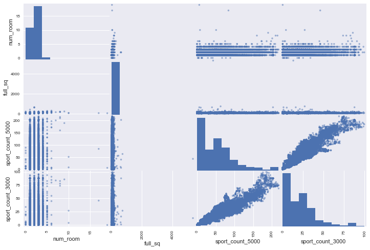
# correlations between most important features

attributes = ["num_room", "full_sq", "sport_count_5000", "sport_count_3000"]
pd.plotting.scatter_matrix(X_train[attributes], figsize=(12,8))

1
2
3
4
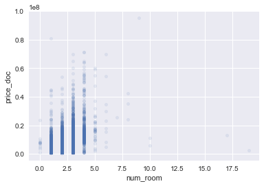
# most interesting is the num_room, so let's plot it against the target feature
# as we can see 

X_train.plot(kind="scatter", x="num_room", y="price_doc", alpha=0.1)

1
2
3
4
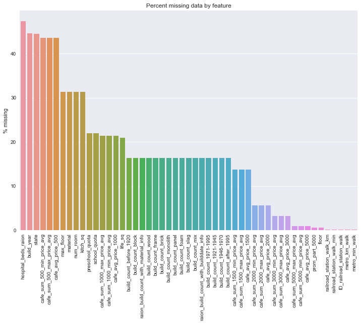
# missing data

train_na = (X_train.isnull().sum() / len(X_train)) * 100 # see the percentage
train_na = train_na.drop(train_na[train_na == 0].index).sort_values(ascending=False) # drop the ones that are zeros

1
2
3
4
5
6
# plot the missing data

f, ax = plt.subplots(figsize=(12, 8))
plt.xticks(rotation='90')
sns.barplot(x=train_na.index, y=train_na)
ax.set(title='Percent missing data by feature', ylabel='% missing')

1
2
3
4
5
6
7
8
# fill the na and get dummy variables from categorical data

X_all = pd.concat(objs = [X_train, X_test], axis=0)
assert isinstance(X_all, pd.DataFrame)

X_all["timestamp"] = X_all["timestamp"].apply(lambda row: str(row).split("-")[0])
X_all.fillna(X_all.mean(), inplace = True)
X_all = pd.get_dummies(X_all)

1
2
3
4
5
6
7
8
9
10
# feature scaling

from sklearn_pandas import DataFrameMapper
from sklearn.preprocessing import StandardScaler

ids = X_all["id"]
mapper = DataFrameMapper([(X_all.columns, StandardScaler())])
scaled_features = mapper.fit_transform(X_all.copy())
scaled_features_df = pd.DataFrame(scaled_features, index=X_all.index, columns=X_all.columns)
scaled_features_df.head()

	0_13_all	0_13_female	0_13_male	0_17_all	0_17_female	0_17_male	0_6_all	0_6_female	0_6_male	16_29_all	...	thermal_power_plant_raion_no	thermal_power_plant_raion_yes	timestamp_2011	timestamp_2012	timestamp_2013	timestamp_2014	timestamp_2015	timestamp_2016	water_1line_no	water_1line_yes
0	1.201285	1.162229	1.235537	1.188467	1.149805	1.222768	1.153571	1.164018	1.141788	-0.223144	...	0.23946	-0.23946	7.045668	-0.381237	-0.51436	-0.74719	-0.47077	-0.341515	0.286628	-0.286628
1	0.523683	0.554055	0.494024	0.548430	0.565753	0.531123	0.445573	0.478837	0.413604	-0.262330	...	0.23946	-0.23946	7.045668	-0.381237	-0.51436	-0.74719	-0.47077	-0.341515	0.286628	-0.286628
2	0.182887	0.138965	0.223825	0.243104	0.199688	0.283535	0.182700	0.137060	0.225079	-0.191497	...	0.23946	-0.23946	7.045668	-0.381237	-0.51436	-0.74719	-0.47077	-0.341515	0.286628	-0.286628
3	2.065314	2.071514	2.055203	2.105747	2.095231	2.111937	2.075597	2.121536	2.029025	-0.460802	...	0.23946	-0.23946	7.045668	-0.381237	-0.51436	-0.74719	-0.47077	-0.341515	0.286628	-0.286628
4	0.235031	0.159379	0.305712	0.281378	0.213312	0.344959	0.137269	0.104510	0.167657	-0.429507	...	0.23946	-0.23946	7.045668	-0.381237	-0.51436	-0.74719	-0.47077	-0.341515	0.286628	-0.286628

5 rows × 459 columns

1
2
3
4
5
6
7
8
9
10
# split the data

X_train = pd.DataFrame(X_all[:len(X_train)])
X_test = pd.DataFrame(X_all[len(X_train):])
length = len(X_train)

y = X_train["price_doc"]

    
X_train_transformed = X_train.drop(["price_doc"], axis = 1).copy()

1
2
X_matrix = X_train_transformed.as_matrix()
y_matrix = y.as_matrix()

1
2
3
4
5
6
# test it with linear regression

from sklearn.linear_model import LinearRegression

lr_clf = LinearRegression()
lr_clf.fit(X_train_transformed, y)

1
2
3
4
5
6
# display all scores in one go

def display_scores(scores):
    print("Scores:", scores)
    print("Mean:", round(scores.mean()))
    print("Standard deviation:", scores.std())

1
2
3
4
5
from sklearn.model_selection import cross_val_score

lr_scores = cross_val_score(lr_clf,X_train_transformed, y, scoring="neg_mean_squared_error", cv=10)
lr_rmse_scores = np.sqrt(-lr_scores)
display_scores(lr_rmse_scores)

1
2
3
4
5
Scores: [  4.24231011e+06   9.91980367e+06   3.43953083e+06   7.66985806e+09
   7.71852130e+06   3.62683154e+06   3.25531314e+09   3.32414976e+06
   3.42314427e+06   3.91199943e+06]
Mean: 1096477749.0
Standard deviation: 2395858735.05

1
2
3
4
5
6
from sklearn.metrics import mean_squared_error

lr_predictions = lr_clf.predict(X_train_transformed)
lr_mse = mean_squared_error(y, lr_predictions)
lr_smre = np.sqrt(lr_mse)
lr_smre

3468938.7143163057

1
2
3
4
5
6
7
8
9
10
11
12
# predict for test with linear regression

X_test_matrix = X_test.drop(["price_doc"], axis = 1).copy().as_matrix()
y_predictions = lr_clf.predict(X_test_matrix)
y_predictions = y_predictions.round()
linear_results = pd.DataFrame(
    {
        "id": ids[length:],
        "price_doc": y_predictions
    }
)
linear_results.to_csv("data/russian_house_market/linear_results.csv", index=False)

1
2
3
4
5
6
7
8
9
10
11
12
13
14
# gradient boosting

from sklearn.ensemble import GradientBoostingRegressor

gbr = GradientBoostingRegressor()
gbr.fit(X_train_transformed, y)
gbr_predictions = gbr.predict(X_test_matrix)
gbr_results = pd.DataFrame(
    {
        "id": ids[length:],
        "price_doc": gbr_predictions
    }
)
gbr_results.to_csv("data/russian_house_market/gbr_results.csv", index=False)

1
2
3
4
5
6
7
8
9
10
11
12
13
14
# random forest regressor

from sklearn.ensemble import RandomForestRegressor

rfr = RandomForestRegressor()
rfr.fit(X_train_transformed, y)
rfr_predictions = rfr.predict(X_test_matrix)
rfr_results = pd.DataFrame(
    {
        "id": ids[length:],
        "price_doc": rfr_predictions
    }
)
rfr_results.to_csv("data/russian_house_market/rfr_results.csv", index=False)

1
2
3
rfr_scores = cross_val_score(rfr,X_train_transformed, y, scoring="neg_mean_squared_error", cv=10)
rfr_rmse_scores = np.sqrt(-rfr_scores)
display_scores(rfr_rmse_scores)

1
2
3
4
5
    Scores: [ 4028866.76898487  2399962.99959557  2670868.71730077  2653273.81372096
      2688965.95341056  3039268.45804425  2772076.02745459  2517358.66164347
      2498985.05770515  3120309.95459634]
    Mean: 2838994.0
    Standard deviation: 451286.366994

1
2
3
gbr_scores = cross_val_score(gbr,X_train_transformed, y, scoring="neg_mean_squared_error", cv=10)
gbr_rmse_scores = np.sqrt(-gbr_scores)
display_scores(gbr_rmse_scores)

1
2
3
4
5
6
# extreme gradient boosting

from xgboost import XGBRegressor

xgb = XGBRegressor()
xgb.fit(X_train_transformed, y)

1
2
3
4
5
6
7
8
9
10
# xgb with test

xgb_predictions = xgb.predict(X_test_matrix)
xgb_results = pd.DataFrame(
    {
        "id": ids[length:],
        "price_doc": xgb_predictions
    }
)
xgb_results.to_csv("data/russian_house_market/xgb_results.csv", index=False)